#Libraries:
library(rvest)
library(dplyr)
library(ggplot2)
library(shiny)
library(shinydashboard)Objective and Description
So, I’m like so much seeing how good MLB’s Teams are in the season, but we have so many games and stats and different tables that we can become overwhelmed. Therefore, I tried to scrap some baseball reference tables to conciliate in visuals and compare some teams in a better way.
First, I’m gonna load all libraries that have been used.
Scrapping Data
To scrap the data from internet, we need to understand the HTML headers and how to search for them to extract the data.
# Scraping Batting Stats --------------------------------------------------

#Web Page - Batting Stats:
url <- "https://www.baseball-reference.com/leagues/majors/2022.shtml"
webpage <- read_html(url)

#Getting HTML Headers for the Table:
col_names_b <- webpage %>%
  html_nodes("table#teams_standard_batting > thead > tr > th") %>%
  html_attr("data-stat")

#Scraping the Teams Names: between <a>
teams_name_data <- webpage %>%
  html_nodes("table#teams_standard_batting > tbody > tr > th > a") %>%
  html_text() %>% as.data.frame()

#Scraping and Applying the data into a DatafRame object:
data = webpage %>%
  html_nodes("table#teams_standard_batting > tbody > tr > td") %>%
  html_text() %>% matrix(ncol = length(col_names_b) - 1, byrow = TRUE) %>% as.data.frame() %>%
  mutate(id = row_number()) %>%
  filter(id < max(id)) %>% select(-id)


#Binding DFs:
df_batting_stats = cbind(teams_name_data, data)
colnames(df_batting_stats) = col_names_b

df_batting_stats = df_batting_stats %>%
  mutate(batting_avg = as.numeric(batting_avg),
         onbase_perc = as.numeric(onbase_perc),
         runs_per_game = as.numeric(runs_per_game),
         H = as.numeric(H))


# Extracting Schedules Data -----------------------------------------------

teams = c('Arizona Diamondbacks',
          'Atlanta Braves',
          'Baltimore Orioles',
          'Boston Red Sox',
          'Chicago Cubs',
          'Chicago White Sox',
          'Cincinnati Reds',
          'Cleveland Guardians',
          'Colorado Rockies',
          'Detroit Tigers',
          'Houston Astros',
          'Kansas City Royals',
          'Los Angeles Angels',
          'Los Angeles Dodgers',
          'Miami Marlins',
          'Milwaukee Brewers',
          'Minnesota Twins',
          'New York Mets',
          'New York Yankees',
          'Oakland Athletics',
          'Philadelphia Phillies',
          'Pittsburgh Pirates',
          'San Diego Padres',
          'Seattle Mariners',
          'San Francisco Giants',
          'St. Louis Cardinals',
          'Tampa Bay Rays',
          'Texas Rangers',
          'Toronto Blue Jays',
          'Washington Nationals')
team_code = c('ARI',
              'ATL',
              'BAL',
              'BOS',
              'CHC',
              'CHW',
              'CIN',
              'CLE',
              'COL',
              'DET',
              'HOU',
              'KCR',
              'LAA',
              'LAD',
              'MIA',
              'MIL',
              'MIN',
              'NYM',
              'NYY',
              'OAK',
              'PHI',
              'PIT',
              'SDP',
              'SEA',
              'SFG',
              'STL',
              'TBR',
              'TEX',
              'TOR',
              'WSN'
)

#Quantity of Games per Team:
teams_games_n = df_batting_stats %>% select(team_name, G) %>% rename(n_games = G)

#Teams Codes an Names:
df_codes = data.frame(teams, team_code)

#Empty DataFrame for Binding Data of all teams Schedules:
df_schedules = data.frame()

#Looping for Extracting the Data:
for (c in df_codes$team_code) {
  #Adapting the URL:
  url_c <- paste0("https://www.baseball-reference.com/teams/", c, "/2022-schedule-scores.shtml")

  #Temporary Support Variables:
  n_c = teams_games_n %>% filter(team_name == df_codes[df_codes["team_code"] == c][1]) %>% select(n_games) %>% as.numeric()

  #Extracting Informations:
  webpage_temp <- read_html(url_c)

  #Columns Names:
  col_names_temp <- webpage_temp %>%
    html_nodes("table#team_schedule > thead > tr > th") %>%
    html_attr("data-stat")

  #Temprary Dataset:
  data_temp <- webpage_temp %>%
    html_nodes("table#team_schedule > tbody > tr > td") %>%
    html_text()

  #Temporary DataFrame:
  df_temp = data_temp[1:((length(col_names_temp) - 1) * n_c)] %>%
    matrix(ncol = length(col_names_temp) - 1, byrow = TRUE)

  #Adding all together:
  final_temp <- as.data.frame(df_temp, stringsAsFactors = FALSE)
  names(final_temp) <- col_names_temp[-1]

  #Final Result:
  final_temp = final_temp %>%
    rename(team_code = team_ID) %>%
    inner_join(df_codes, by = "team_code")

  #Binding Rows:
  df_schedules = rbind(df_schedules, final_temp)

  #Cleaning Env. Variables:
  rm(url_c,
     n_c,
     webpage_temp,
     data_temp,
     df_temp,
     final_temp)
}

#Fooling Around with the Schedules Dataset:
df_schedules = df_schedules %>%
  mutate(game_date_adj = if_else(stringr::str_sub(stringr::str_trim(date_game, "both"), -3, -1) %in% c("(1)", "(2)", "(3)"),
                                 stringr::str_trim(stringr::str_sub(date_game, 1, -4), "both"),
                                 stringr::str_trim(date_game, "both")),
         flag_win = if_else(stringr::str_detect(win_loss_result, "W"), 1, 0)) %>%
  tidyr::separate(game_date_adj, sep = ",", into = c("weekd", "mmdd")) %>%
  mutate(date_format1 = paste0(stringr::str_trim(mmdd, "both"), " 2022")) %>%
  tidyr::separate(date_format1, into = c("month", "day", "year"), sep = " ") %>%
  mutate(month2 = match(month, month.abb),
         date2 = paste(day, month2, year, sep = "/")) %>%
  mutate(date_format = as.Date(date2, "%d/%m/%Y"))
In the previous code, we ware looking for the tables headers to scrap the offense stats by every team, and after that we are looking for the schedule of each team and getting the data available, this data is good for understanding the teams recent runs pattern, since we have a lot of games in MLB season.
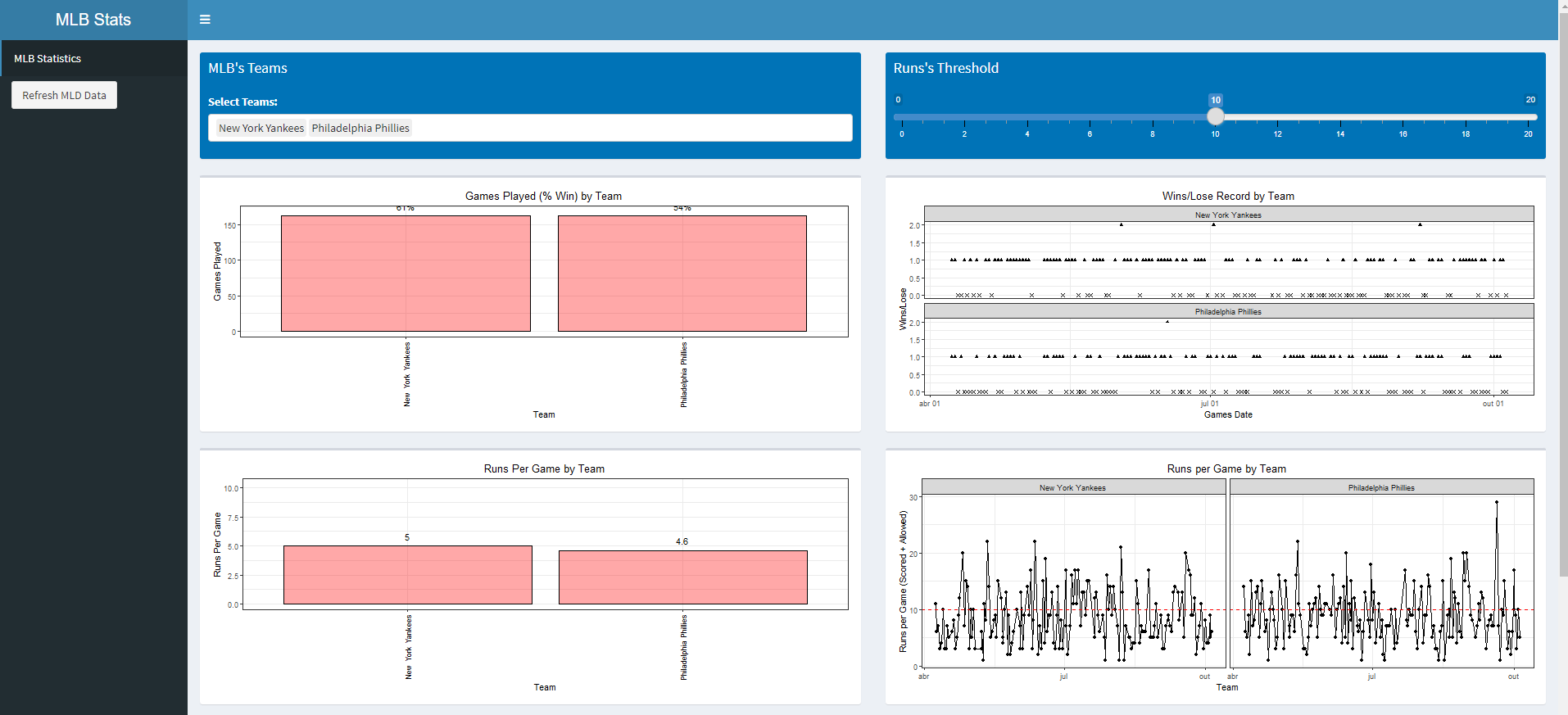
Building the visuals and the Shiny App
Now that we have our data, the easy part is building the visual to help us analyze this data.
# Shiny App Section -------------------------------------------------------
#Shiny App:
ui <- dashboardPage(
#DashBoard Header:
dashboardHeader(title = "MLB Stats"),
#Dashboard Sidebar:
dashboardSidebar(
sidebarMenu(
menuItem("MLB Statistics", tabName = "stats"),
actionButton("refresh-data", "Refresh MLD Data")
)),
#DashBoard Body:
dashboardBody(tabItems(
# Teams Stats Content:
tabItem(tabName = "stats",
fluidRow(
box(
title = "MLB's Teams", background = "blue",
selectInput("select_team", "Select Teams:", multiple = T, choices = unique(df_batting_stats$team_name), selected = "New York Yankees"),
width = 6, height = 130),
box(
title = "Runs's Threshold", background = "blue",
sliderInput("select_th", label = NULL, min = 0, max = 20, value = 10),
width = 6, height = 130)
),
#First Row of Plots:
fluidRow(
box(
plotOutput("plot_g5", width = NULL, height = 290)
),
box(
plotOutput("plot_g6", width = NULL, height = 290)
)
),
#Second Row of Plots:
fluidRow(
box(
plotOutput("plot_g1", width = NULL, height = 290)
),
box(
plotOutput("plot_g2", width = NULL, height = 290)
)
),
#Third Row of Plots:
fluidRow(
box(
plotOutput("plot_g3", width = NULL, height = 290)
),
box(
plotOutput("plot_g4", width = NULL, height = 290)
)
)
)
))
)
server <- function(input, output) {
#Plot 5: Graph
output$plot_g5 <- renderPlot({
df_schedules %>%
filter(teams %in% input$select_team) %>%
group_by(teams) %>%
summarise(Games = n(),
Wins = sum(flag_win)) %>%
mutate(win_pctg = Wins/Games) %>%
ggplot(aes(x = teams, y = Games, label = paste0(round(win_pctg*100, 0), "%"))) +
geom_bar(stat = "identity", col = 'black', fill = "red", alpha = 0.34) +
theme_bw() +
ylim(c(0, as.numeric(max(teams_games_n$n_games)) + 5)) +
geom_text(vjust = -0.8) +
labs(x = "Team", y = "Games Played", title = "Games Played (% Win) by Team") +
theme(axis.text.x = element_text(angle = 90, vjust = 0.5, color = "black"), plot.title = element_text(hjust = 0.5))
})
#Plot 6: Graph
output$plot_g6 <- renderPlot({
df_schedules %>%
filter(teams %in% input$select_team) %>%
group_by(teams, date_format) %>%
summarise(wins = sum(flag_win)) %>%
group_by(teams, date_format) %>% ungroup() %>%
mutate(date_format = lubridate::ymd(date_format),
tp = if_else(wins > 0, "win", "lose")) %>%
ggplot(aes(x = date_format, y = wins, shape = tp)) +
geom_point() +
scale_shape_manual("", values = c(win = 17, lose = 4), guide = "none") +
scale_x_date(date_labels = "%b %d") +
facet_wrap(~teams, ncol = 1) +
theme_bw() +
labs(x = "Games Date", y = "Wins/Lose", title = "Wins/Lose Record by Team") +
theme(legend.position = "none",
plot.title = element_text(hjust = 0.5))
})
#Plot 1: Graph
output$plot_g1 <- renderPlot({
df1 = df_batting_stats %>% filter(team_name %in% input$select_team)
df1 %>%
ggplot(aes(x = team_name, y = runs_per_game, label = round(runs_per_game, 1))) +
geom_bar(stat = "identity", col = 'black', fill = "red", alpha = 0.34) +
theme_bw() +
geom_text(vjust = -0.8) +
ylim(c(0, max(df_batting_stats$runs_per_game) + 5)) +
labs(x = "Team", y = "Runs Per Game", title = "Runs Per Game by Team") +
theme(axis.text.x = element_text(angle = 90, vjust = 0.5, color = "black"), plot.title = element_text(hjust = 0.5))
})
#Plot 2: Graph Substirutir por serie temporal
output$plot_g2 <- renderPlot({
df2 = df_schedules %>% filter(teams %in% input$select_team) %>%
mutate(runs = as.numeric(R) + as.numeric(RA))
df2 %>%
ggplot(aes(x = date_format, y = runs)) +
geom_point() +
geom_line() +
theme_bw() +
facet_wrap(~teams) +
labs(x = "Team", y = "Runs per Game (Scored + Allowed)", title = "Runs per Game by Team") +
geom_hline(yintercept = input$select_th, linetype = 2, col = "red") +
theme(plot.title = element_text(hjust = 0.5))
})
#Plot 3: Graph
output$plot_g3 <- renderPlot({
df3 = df_batting_stats %>% filter(team_name %in% input$select_team)
df3 %>%
ggplot(aes(x = H, y = runs_per_game, label = team_name, col = onbase_perc)) +
geom_point() +
geom_text(vjust = -0.8) +
theme_bw() +
ylim(c(0, max(df_batting_stats$runs_per_game) + 5)) +
xlim(c(min(df_batting_stats$H) - 10, max(df_batting_stats$H) + 10)) +
geom_hline(yintercept = mean(df_batting_stats$runs_per_game), linetype = 2, col = "red") +
geom_vline(xintercept = mean(df_batting_stats$H), linetype = 2, col = "red") +
labs(x = "Total Hits", y = "Runs Per Game", title = "Runs Per Game x Hits (+ On Base %)") +
theme(plot.title = element_text(hjust = 0.5))
})
#Plot 4: Graph
output$plot_g4 <- renderPlot({
df_schedules %>%
filter(teams %in% input$select_team) %>%
group_by(teams, date_format) %>%
summarise(avg_runs_scored = mean(as.numeric(R), na.rm = T),
avg_runs_allow = mean(as.numeric(RA), na.rm = T)) %>% ungroup() %>%
mutate(date_format = lubridate::ymd(date_format)) %>%
tidyr::pivot_longer(cols = starts_with("avg"), names_to = "cat", values_to = "avg") %>%
ggplot(aes(x = cat, y = avg, fill = cat)) +
geom_boxplot() +
facet_wrap(~teams) +
theme_bw() +
labs(x = "Stat", y = "Average Value", title = "Average Scores per Team") +
theme(legend.position = "none",
plot.title = element_text(hjust = 0.5))
})
}
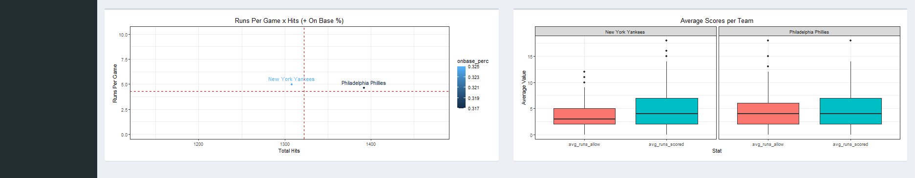
#shinyApp(ui, server) I dont't want to deploy the appResult
This is the result of the shiny app.